Analysis shows how to get the best results when approximating solutions to complex engineering problems.
Optimization algorithms, which try to find the minimum values of mathematical functions, are everywhere in engineering. Among other things, they’re used to evaluate design tradeoffs, to assess control systems, and to find patterns in data.
One way to solve a difficult optimization problem is to first reduce it to a related but much simpler problem, then gradually add complexity back in, solving each new problem in turn and using its solution as a guide to solving the next one. This approach seems to work well in practice, but it’s never been characterized theoretically.
This month, at the International Conference on Energy Minimization Methods in Computer Vision and Pattern Recognition, Hossein Mobahi, a postdoc at MIT’s Computer Science and Artificial Intelligence Laboratory (CSAIL), and John Fisher, a senior research scientist at CSAIL, describe a way to generate that sequence of simplified functions that guarantees the best approximation that the method can offer.
“There are some fundamental questions about this method that we answer for the first time,” Mobahi says. “For example, I told you that you start from a simple problem, but I didn’t tell you how you choose that simple problem. There are infinitely many functions you can start with. Which one is good? Even if I tell you what function to start with, there are infinitely many ways to transform that to your actual problem. And that transformation affects what you get at the end.”
Bottoming out
To get a sense of how optimization works, suppose that you’re a canned-food retailer trying to save money on steel, so you want a can design that minimizes the ratio of surface area to volume. That ratio is a function of the can’s height and radius, so if you can find the minimum value of the function, you’ll know the can’s optimal dimensions. If you’re a car designer trying to balance the costs of components made from different materials with the car’s weight and wind resistance, your function — known in optimization as a “cost function” — will be much more complex, but the principle is the same.
Machine-learning algorithms frequently attempt to identify features of data sets that are useful for classification tasks — say, visual features characteristic of cars. Finding the smallest such set of features with the greatest predictive value is also an optimization problem.
“Most of the efficient algorithms that we have for solving optimization tasks work based on local search, which means you initialize them with some guess about the solution, and they try to see in which direction they can improve that, and then they take that step,” Mobahi says. “Using this technique, they can converge to something called a local minimum, which means a point that compared to its neighborhood is lower. But it may not be a global minimum. There could be a point that is much lower but farther away.”
A local minimum is guaranteed to be a global minimum, however, if the function is convex, meaning that it slopes everywhere toward its minimum. The function y = x2 is convex, since it describes a parabola centered at the origin. The function y = sin x is not, since it describes a sine wave that undulates up and down.
Smooth sailing
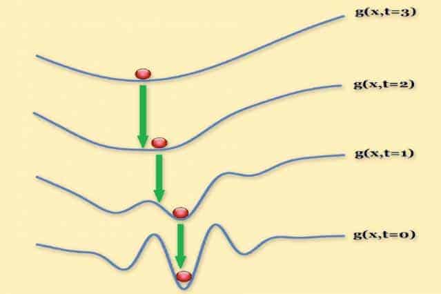
Mobahi and Fisher’s method begins by trying to find a convex approximation of an optimization problem, using a technique called Gaussian smoothing. Gaussian smoothing converts the cost function into a related function that gives not the value that the cost function would, but a weighted average of all the surrounding values. This has the effect of smoothing out any abrupt dips or ascents in the cost function’s graph.
The weights assigned the surrounding values are determined by a Gaussian function, or normal distribution — the bell curve familiar from basic statistics. Nearby values count more toward the average than distant values do.
A Gaussian function is defined by a single parameter, which determines its width. Mobahi and Fisher begin with a very wide Gaussian, which, under certain conditions, yields a convex function. Then they steadily contract the width of the Gaussian, generating a series of intermediary problems. At each stage, they use the solution to the last problem to initialize the search for a solution to the next one. By the time the width of the distribution has shrunk to zero, they’ve recovered the original cost function, since every value is simply the average of itself.
“The continuation method for optimization is something that is really widely used in practice, widely used in computer vision, for solving alignment problems, for solving tracking problems, a bunch of different places, but it’s not very well understood,” says John Wright, an assistant professor of electrical engineering at Columbia University who was not involved in this work. “The interesting thing about Hossein’s work in general, and this paper in particular, is that he’s really digging into this continuation method and trying to see what we can say analytically about this.”
“The practical utility of that is, there might be any number of different ways that you could go about doing smoothing or trying to do coarse-to-fine optimization,” Wright adds. “If you know ahead of time that there’s a right one, then you don’t waste a lot of time pursuing the wrong ones. You have a recipe rather than having to look around.”


